---

Generating Pink Noise Using Python

Pink noise, also known as 1/f noise, is a type of random signal that has equal energy per octave. Unlike white noise, which has a constant power spectral density across all frequencies, pink noise decreases in power as the frequency increases. It is commonly used in audio applications, such as sound masking, music production, and testing audio equipment.

Here’s what it sounds like:

In this blog post, we’ll walk through a Python function that generates pink noise and saves it to a WAV file. Disclaimer, the audio above is an mp3 after I converted the .wav file to an mp3.

I wanted to add that “Pink Noise” seems to be something that is naturally occurring in nature as well!

Pink noise includes a variety of natural sounds including steady rain, the wind in the trees and running water in a river or stream. It is also the deep sound of a human heartbeat. Many people have found that Pink Noise can help them to concentrate and improves memory and information retention.

https://silvotherapy.co.uk/articles/white-noise-brown-noise-and-nature

The Code

import numpy as np
from scipy.io import wavfile

def generate_pink_noise(n_samples, sample_rate):
    # Generate white noise
    white_noise = np.random.randn(n_samples)
    
    # Compute FFT of white noise
    white_fft = np.fft.rfft(white_noise)
    
    # Compute frequency bins
    freqs = np.fft.rfftfreq(n_samples, d=1/sample_rate)
    
    # Compute scaling factors for each frequency bin to create pink noise
    scale = np.zeros_like(freqs)
    scale[1:] = 1 / np.sqrt(freqs[1:])  # Exclude DC component
    
    # Apply scaling to FFT of white noise
    pink_fft = white_fft * scale
    
    # Inverse FFT to obtain pink noise
    pink_noise = np.fft.irfft(pink_fft)
    
    # Normalize to 16-bit range
    pink_noise *= 32767 / np.max(np.abs(pink_noise))
    
    return pink_noise.astype(np.int16)

# Generate pink noise
sample_rate = 44100
duration = 10  # seconds
n_samples = sample_rate * duration

pink = generate_pink_noise(n_samples, sample_rate)

# Save pink noise to WAV file
wavfile.write('pink_noise.wav', sample_rate, pink)

print("Pink noise generated and saved to 'pink_noise.wav'.")

How It Works

1. We start by generating white noise using np.random.randn(n_samples). White noise is a random signal with a flat power spectral density across all frequencies.
2. Next, we compute the FFT (Fast Fourier Transform) of the white noise using np.fft.rfft(white_noise). This gives us the frequency domain representation of the signal.
3. We calculate the frequency bins using np.fft.rfftfreq(n_samples, d=1/sample_rate). These represent the different frequencies in our signal.
4. To create pink noise, we compute scaling factors for each frequency bin. The scaling factors decrease with increasing frequency, following a 1/f relationship. We exclude the DC component (bin 0) from scaling.
5. We apply the scaling factors to the FFT of white noise, resulting in the pink noise FFT.
6. Finally, we perform an inverse FFT on the pink noise FFT to obtain the time-domain pink noise signal.
7. The pink noise is then normalized to fit within the 16-bit range for audio data.

Now you know how to generate pink noise in Python! Feel free to experiment with different parameters, such as sample rate and duration, to create custom pink noise for your projects.

Keep in mind you need to install numpy, scipy and matplotlib for this to work!

Remember to save the generated pink noise to a WAV file (like I did with ‘pink_noise.wav’) for practical use. I also converted it to an mp3 as I mentioned earlier but this was because it’s much easier to run FFT analysis on .wav files than it is for .mp3 files. Remember, .wav is raw audio and .mp3 files are compressed.

---

Analyzing Pink Noise: FFT Magnitude

Above, we generated pink noise and saved it to a WAV file. Now, let’s explore how to analyze this audio signal using Python to verify if it’s actually Pink noise.

The New Code

import numpy as np
from scipy.io import wavfile
import matplotlib.pyplot as plt

""" 
This script reads in a wav file, runs an FFT against it, 
and then stores the magnitude plot as a .png image
"""

def analyze_wav_file(file_name):
    sample_rate, data = wavfile.read(file_name)

    # Perform the FFT
    fft_result = np.fft.fft(data)

    # Get real and imaginary parts
    real_part = np.real(fft_result)
    imag_part = np.imag(fft_result)

    # Calculate magnitude
    magnitude = np.sqrt(real_part**2 + imag_part**2)

    # Convert magnitude to dB (To plot a log)
    magnitude_db = 20 * np.log10(magnitude)

    # Create frequency axis
    freq = np.fft.fftfreq(len(magnitude), 1/sample_rate)

    # Only keep positive frequencies
    positive_freq_mask = freq >= 0
    freq = freq[positive_freq_mask]
    magnitude_db = magnitude_db[positive_freq_mask]

    # Plot the magnitude in dB
    plt.figure(figsize=(12, 6))
    plt.plot(freq, magnitude_db)
    plt.title(f'FFT Magnitude (dB) for {file_name}')
    plt.xlabel('Frequency [Hz]')
    plt.ylabel('Magnitude [dB]')
    plt.savefig(f'magnitude_{file_name}.png')  # Save the figure as 'magnitude.png'
    plt.close()  # Close the figure to free up memory

# Read the .wav file
file_name = 'pink_noise.wav'
analyze_wav_file(file_name)

How It Works

1. Reading the WAV File: We start by reading the pink noise WAV file using wavfile.read(file_name). This gives us the sample rate and the audio data.
2. FFT (Fast Fourier Transform): We compute the FFT of the audio data using np.fft.fft(data). This transforms the time-domain signal into the frequency domain.
3. Magnitude: We extract the real and imaginary parts from the FFT result. The magnitude is calculated as the square root of the sum of squares of the real and imaginary parts.
4. Magnitude in dB: To visualize the magnitude, we convert it to decibels (dB) using 20 * np.log10(magnitude). This allows us to plot it on a logarithmic scale.
5. Frequency Axis: We create a frequency axis using np.fft.fftfreq(len(magnitude), 1/sample_rate).
6. Positive Frequencies Only: We keep only the positive frequencies (since the FFT result is symmetric). Otherwise, we get a mirrored version on the left.
7. Plotting: We plot the magnitude in dB against frequency. The resulting plots are saved as PNG images.

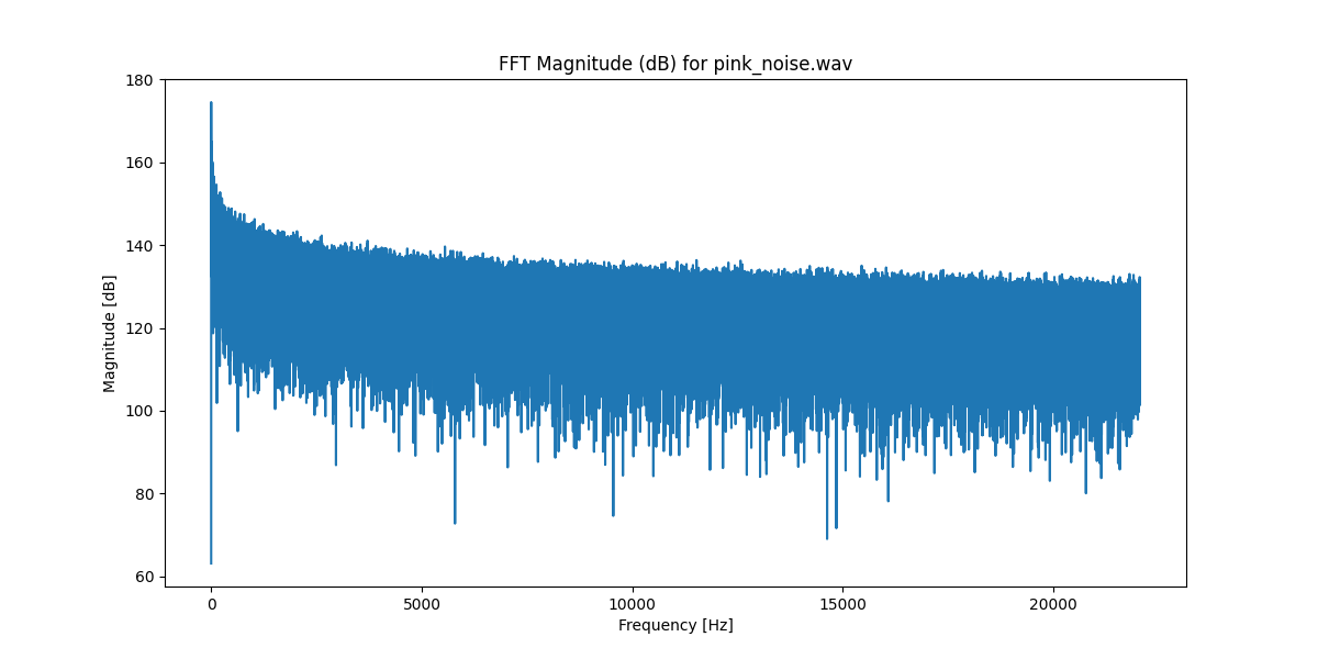
Running the generated pink noise file through the above script, generates this plot:

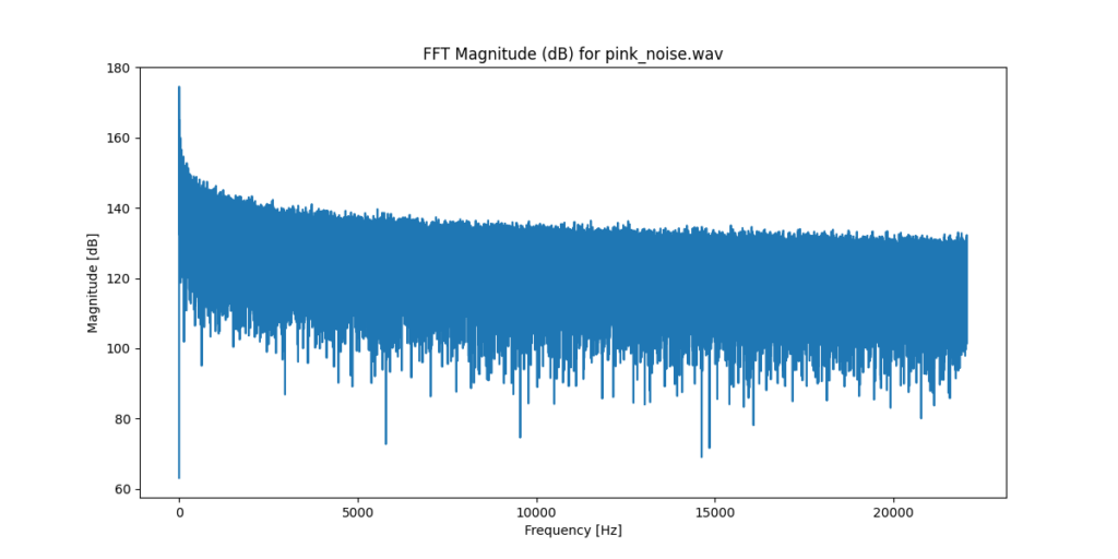
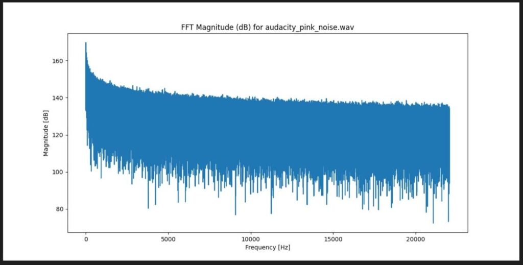
Very impressive!! This is promising since generating Pink noise using Audacity gives us the following plot which is very similar!

Conclusion

By analyzing the FFT magnitude, we gain insights into the frequency components of the pink noise.

All of this code can be found in my GitHub here: https://github.com/sigmaenigma/SoundProcessing/tree/main

Happy coding! d-_-b